Superposition of Pharmacokinetic Data

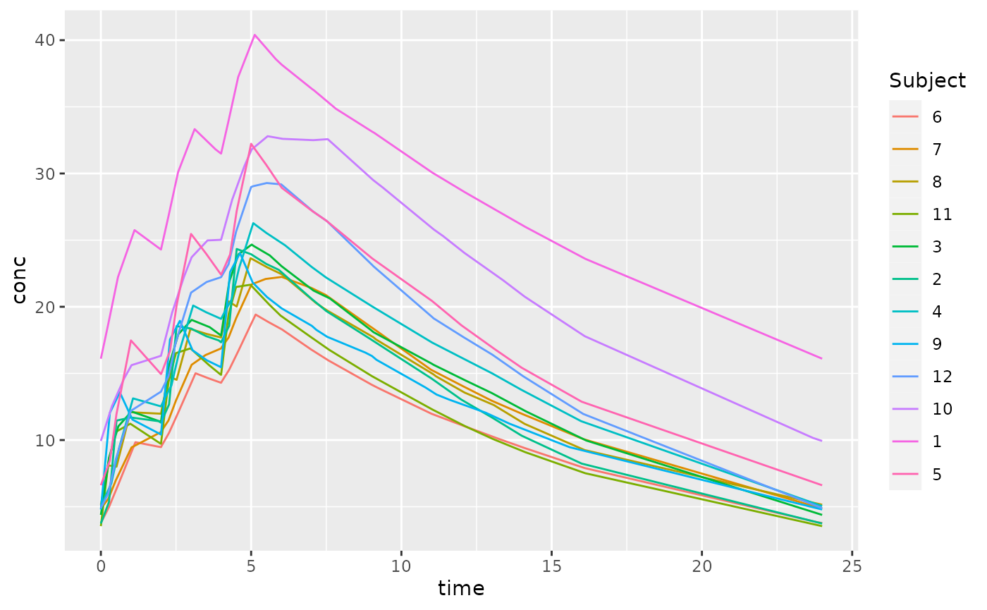
Examples simplify understanding. Below is an example of how to use the theophylline dataset to estimate the concentration for each subject after multiple doses.

Load the data

## It is always a good idea to look at the data
knitr::kable(head(datasets::Theoph))

Subject	Wt	Dose	Time	conc
1	79.6	4.02	0.00	0.74
1	79.6	4.02	0.25	2.84
1	79.6	4.02	0.57	6.57
1	79.6	4.02	1.12	10.50
1	79.6	4.02	2.02	9.66
1	79.6	4.02	3.82	8.58

The columns that we will be interested in for our analysis are conc, Time, and Subject in the concentration data.

## By default it is groupedData; convert it to a data frame for use
conc_obj <- PKNCAconc(as.data.frame(datasets::Theoph), conc~Time|Subject)

Compute the Superposition from Single-Dose Data to Steady-State

With a simple call, we can have the estimated steady-state concentration for each subject. At minimum, the time between dosing (tau) must be provided.

steady_state <- superposition(conc_obj, tau=24)

## Warning in parallel::mclapply(X = seq_len(nrow(nested_data)), FUN =
## function(idx) {: all scheduled cores encountered errors in user code

The error noting that the first concentration must be zero is due to the fact that superposition usually occurs with single-dose data. If the first concentration is nonzero, the data are not likely to be single-dose (or a data error should be fixed). Let’s find the offending data.

knitr::kable(subset(datasets::Theoph, Time == 0 & conc > 0),
             caption="Nonzero predose measurements",
             row.names=FALSE)

Nonzero predose measurements
Subject	Wt	Dose	conc
1	79.6	4.02	0.74
7	64.6	4.95	0.15
10	58.2	5.50	0.24

For this example, we will assume that these were errors, correct them to zero, and recalculate.

## Correct nonzero concentrations at time 0 to be BLQ.
theoph_corrected <- as.data.frame(datasets::Theoph)
theoph_corrected$conc[theoph_corrected$Time == 0] <- 0
conc_obj_corrected <- PKNCAconc(theoph_corrected, conc~Time|Subject)

## Calculate the new steady-state concentrations with 24 hour dosing
steady_state <- superposition(conc_obj_corrected, tau=24)
knitr::kable(head(steady_state, n=14),
             caption="Superposition at steady-state")

Superposition at steady-state
Subject	conc	time
1	4.856234	0.00
1	7.637741	0.25
1	9.008665	0.37
1	11.293912	0.57
1	15.099676	1.12
1	14.063389	2.02
1	12.615588	3.82
1	12.152885	5.10
1	10.924249	7.03
1	10.022157	9.05
1	8.639209	12.12
1	4.857207	24.00
2	1.010060	0.00
2	2.703513	0.27

The output is a tbl_df, tbl, data.frame including all the grouping factors as columns, a column for concentration, and a column for time. Time point selection ensures that the beginning and end of the interval are included and that every measured time that contributes to the interval is included. The points at the beginning and end of the interval are very similar; they are within a tolerance of 0.001 as defined by the steady.state.tol argument to superposition.

Nonstandard Superposition Computations

Compute the Superposition from Single-Dose Data to a Specific Dose

If simulation to a specific dose is needed, the number of dosing intervals (n.tau) can be specified.

## Calculate the unsteady-state concentrations with 24 hour dosing
unsteady_state <- superposition(conc_obj_corrected, tau=24, n.tau=2)
knitr::kable(head(unsteady_state, n=14),
             caption="Superposition before steady-state")

Superposition before steady-state
Subject	conc	time
1	3.3393647	0.00
1	6.1391369	0.25
1	7.5187500	0.37
1	9.8183657	0.57
1	13.6629359	1.12
1	12.6879608	2.02
1	11.3550445	3.82
1	10.9681517	5.10
1	9.8452907	7.03
1	9.0438064	9.05
1	7.7960929	12.12
1	4.3830987	24.00
2	0.9268958	0.00
2	2.6226541	0.27

Compute the Superposition from Single-Dose Data with >1 Dose Per Interval

Some dosing intervals are more complex than once per X hours (or days or weeks or…). To predict more complex dosing with superposition, give the dose times within the interval. The dose.times must all be less than tau (otherwise they are not in the interval).

## Calculate the new steady-state concentrations with 24 hour dosing
complex_interval_steady_state <- superposition(conc_obj_corrected, tau=24, dose.times=c(0, 2, 4))
knitr::kable(head(complex_interval_steady_state, n=10),
             caption="Superposition at steady-state with complex dosing")

Superposition at steady-state with complex dosing
Subject	conc	time
1	16.10210	0.00
1	18.74815	0.25
1	20.05464	0.37
1	22.23332	0.57
1	25.75130	1.12
1	24.29240	2.00
1	24.48753	2.02
1	26.79323	2.25
1	28.03334	2.37
1	30.10259	2.57

ggplot(complex_interval_steady_state,
       aes(y=conc, x=time, colour=Subject)) +
  geom_line()

With this more complex dosing interval, the number of time points estimated increases. The next section describes the selection of time points.

Show the Curve to Steady-State

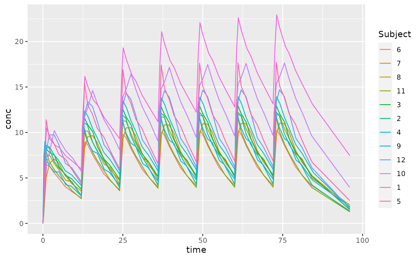
To determine the concentration curve to get to steady-state, you can give all the dose times considered required to get to steady-state. To do this, specify tau as the total time to steady-state, specify n.tau as 1 to indicate that only one round of dosing should be administered.

This command does not technically go to steady-state; if the dose.times are not sufficiently long to reach steady-state, it only goes for as many doses as requested.

up_to_steady_state <- superposition(conc_obj_corrected,
                                    tau=4*24,
                                    n.tau=1,
                                    dose.times=seq(0, 3*24, by=12))

ggplot(up_to_steady_state, aes(x=time, y=conc, colour=Subject)) +
  geom_line()

Time Point Selection and Addition

Superposition is often used to estimate NCA parameters with nonparametric methods. To ensure that estimated parameters are as accurate as possible (especially \(C_{max}\)), each dose has every post-dose time point included. Specifically, each dose will have the following times:

0 (zero) and tau,
The time of each dose (the dose.times argument)
Every value from the time column of the data modulo tau (shifting the time for each measurement to be within the dosing interval) repeated for each dose, and
each time from the additional.times argument.

How the number of time points increases can be seen by comparing the time points for subject 1 in the steady-state single dosing and the complex dosing examples above.

steady_state$time[steady_state$Subject == 1]

##  [1]  0.00  0.25  0.37  0.57  1.12  2.02  3.82  5.10  7.03  9.05 12.12 24.00

sum(steady_state$Subject == 1)

## [1] 12

complex_interval_steady_state$time[complex_interval_steady_state$Subject == 1]

##  [1]  0.00  0.25  0.37  0.57  1.12  2.00  2.02  2.25  2.37  2.57  3.12  3.82
## [13]  4.00  4.02  4.25  4.37  4.57  5.10  5.12  5.82  6.02  7.03  7.10  7.82
## [25]  9.03  9.05  9.10 11.03 11.05 12.12 13.05 14.12 16.12 24.00

sum(complex_interval_steady_state$Subject == 1)

## [1] 34

Interpolation and Extrapolation Methods

The interpolation and extrapolation methods align with those used for calculating the AUC. By default, interpolation uses the PKNCA.options selection for "auc.method" and extrapolation follows the curve of \(AUC_{inf}\). These can be modified with the interp.method and extrap.method arguments.

Bill Denney