Noncompartmental evaluation of time to steady-state

Bill Denney

2024-11-05

Time to steady-state (TSS) can be estimated with PKNCA using either a monoexponential increase toward an asymptote or by a linear regression of the last points. According to Maganti (2008), the monoexponential method is preferred.

TSS can be estimated using either method using the pk.tss() function in PKNCA.

Example

Data setup

Illustrating time to steady-state, the example from the superposition vignette will be used.

library(PKNCA)
theoph_corrected <- as.data.frame(datasets::Theoph)
theoph_corrected$conc[theoph_corrected$Time == 0] <- 0
conc_obj <- PKNCAconc(theoph_corrected, conc~Time|Subject)
steady_state <- superposition(conc_obj, dose.times = seq(0, 168 - 12, by=12), tau=168, n.tau=1)
# Add some noise to the data so that it seems more reasonable
steady_state_noise <- steady_state
steady_state_noise$conc <-
  withr::with_seed(
    seed = 5,
    steady_state_noise$conc*exp(rnorm(nrow(steady_state_noise), mean = 0, sd = 0.1))
  )

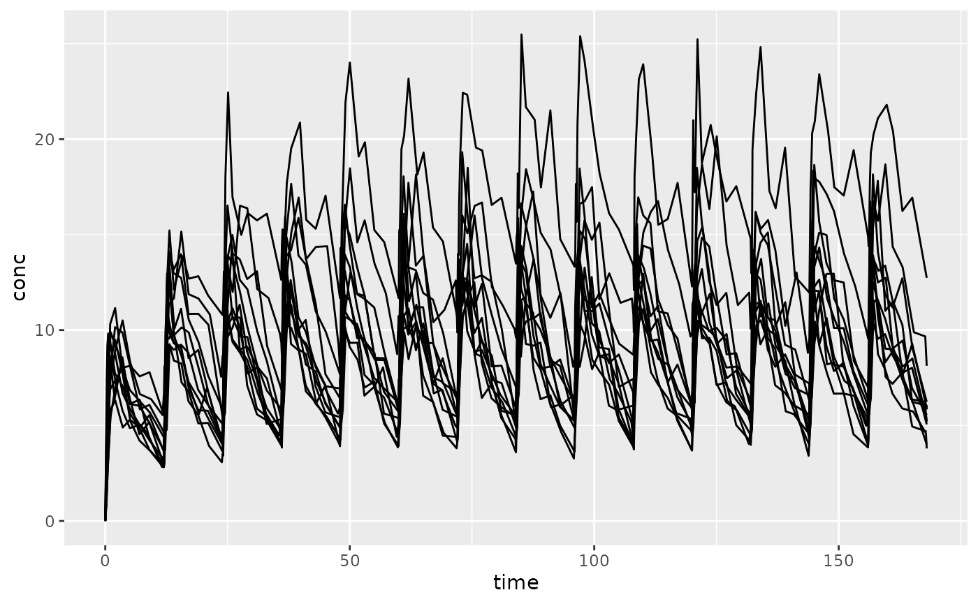
Examine the data graphically.

library(ggplot2)
ggplot(steady_state_noise, aes(x=time, y=conc, groups=Subject)) + geom_line()

Estimate time to Steady State

Monoexponential

The below code estimates four different types of monoexponential time to steady-state:

1. tss.monoexponential.population: The population estimate of TSS using a nonlinear mixed effects model (one value for all subjects)
2. tss.monoexponential.popind: The individual estimate from a nonlinear mixed effects model (one value per subject)
3. tss.monoexponential.individual: The individual estimate using a gnls model to estimate each subject separately (one value per subject)
4. tss.monoexponential.single: The mean estimate of TSS using a nonlinear model

tss_mono <-
  pk.tss.monoexponential(
    conc = steady_state_noise$conc,
    time = steady_state_noise$time,
    subject = steady_state_noise$Subject,
    time.dosing = seq(0, 168 - 12, by=12)
  )
#> Warning in nlme.formula(conc ~ ctrough.ss * (1 - exp(tss.constant * time/tss)),
#> : Iteration 1, LME step: nlminb() did not converge (code = 1). Do increase
#> 'msMaxIter'!
tss_mono
#>    subject tss.monoexponential.population tss.monoexponential.popind
#> 1        1                       26.41698                   36.94302
#> 2       10                       26.41698                   31.95467
#> 3       11                       26.41698                   22.79693
#> 4       12                       26.41698                   26.59837
#> 5        2                       26.41698                   23.53946
#> 6        3                       26.41698                   24.72265
#> 7        4                       26.41698                   25.73792
#> 8        5                       26.41698                   26.93388
#> 9        6                       26.41698                   23.21909
#> 10       7                       26.41698                   25.39792
#> 11       8                       26.41698                   24.54268
#> 12       9                       26.41698                   24.61721
#>    tss.monoexponential.individual tss.monoexponential.single
#> 1                        40.65290                   27.87592
#> 2                        24.72591                   27.87592
#> 3                        20.18663                   27.87592
#> 4                        22.58610                   27.87592
#> 5                        25.45251                   27.87592
#> 6                        29.97015                   27.87592
#> 7                        21.60401                   27.87592
#> 8                        25.04023                   27.87592
#> 9                        23.53884                   27.87592
#> 10                       31.37369                   27.87592
#> 11                       32.02870                   27.87592
#> 12                       26.01334                   27.87592

The fraction of steady-state required for time to steady-state can be changed with the tss.fraction argument (see ?pk.tss.monoexponential).

Stepwise Linear

The stepwise linear method estimates if the slope of the predose concentrations is statistically significant starting from the last measurement and moving backward in time. It has bias in that more individuals will move the time to steady-state to a late time point.

tss_step <-
  pk.tss.stepwise.linear(
    conc = steady_state_noise$conc,
    time = steady_state_noise$time,
    subject = steady_state_noise$Subject,
    time.dosing = seq(0, 168 - 12, by=12)
  )
tss_step
#>   tss.stepwise.linear
#> 1                 108

References

1. Maganti, L., Panebianco, D.L. & Maes, A.L. Evaluation of Methods for Estimating Time to Steady State with Examples from Phase 1 Studies. AAPS J 10, 141–147 (2008). https://doi.org/10.1208/s12248-008-9014-y