Introduction to 'ggtibble'

library(ggtibble)

Motivation for ggtibble

From time to time, having a list of ggplots and being able to work on them like a regular ggplot can be very helpful. For example, when writing a report, you may want to make a set of figures to separate out various levels of a group, then make separate figures for each group.

Introduction

The ggtibble package has two main functions to create sets of figures, ggtibble() and gglist(). These create a tibble with optional labels per figure and captions (for ggtibble()) or a simpler list of figures (for gglist()).

Both ggtibble and gglist objects can have ggplot geoms, facets, labels, and lists of those added to them as though they were normal ggplot objects. And, you can add a gglist to either a ggtibble or a gglist.

Typical use

Typical use will load required libraries, setup your plot data, generate the plot, and then knit_print() it.

When generating the plot:

1. Give your dataset,
2. Indicate your columns for plotting using the aes() mapping as for any ggplot2 object,
3. Provide the outercols which are columns outside your dataset; one plot will be generated for each unique level of your data with the outercols. Note that you cannot use outercols columns within the plot, but you will use them for captions and labels.
4. You can give a caption with a glue::glue_data() specification where valid columns are any column names that are in your outercols specification. (If you don’t give a caption, then it will be an empty string, "".)
5. You can give a list of labels which are each processed the same as the caption via glue::glue_data() and then passed to labs().
6. After the plot is setup in ways that are specific to ggtibble, use it like a normal ggplot object adding geoms, etc.

# Note, add `fig.cap=all_plots$caption` to show the generated caption for the
# figures

library(ggtibble)
library(dplyr)
#> 
#> Attaching package: 'dplyr'
#> The following objects are masked from 'package:stats':
#> 
#>     filter, lag
#> The following objects are masked from 'package:base':
#> 
#>     intersect, setdiff, setequal, union
library(ggplot2)
#> 
#> Attaching package: 'ggplot2'
#> The following objects are masked from 'package:ggtibble':
#> 
#>     %+%, ggsave

d_plot <-
  mtcars |>
  mutate(
    dispu = "cu. in."
  )
all_plots <-
  ggtibble(
    d_plot,
    aes(x = disp, y = hp),
    outercols = c("cyl", "dispu"),
    caption = "Horsepower by displacement for {cyl} cars",
    labs = list(x = "Displacement ({dispu})", y = "Gross horsepower")
  ) +
  geom_point() +
  geom_line()

# The result is a tibble with columns for the `data_plot`, `figure`, and
# `caption`
as_tibble(all_plots)
#> # A tibble: 3 × 5
#>     cyl dispu   data_plot                   figure caption                      
#>   <dbl> <chr>   <list>                    <gglist> <glue>                       
#> 1     6 cu. in. <tibble [7 × 10]>  A ggplot object Horsepower by displacement f…
#> 2     4 cu. in. <tibble [11 × 10]> A ggplot object Horsepower by displacement f…
#> 3     8 cu. in. <tibble [14 × 10]> A ggplot object Horsepower by displacement f…

# You can then show all the figures with the `knit_print()` method.
knit_print(all_plots)

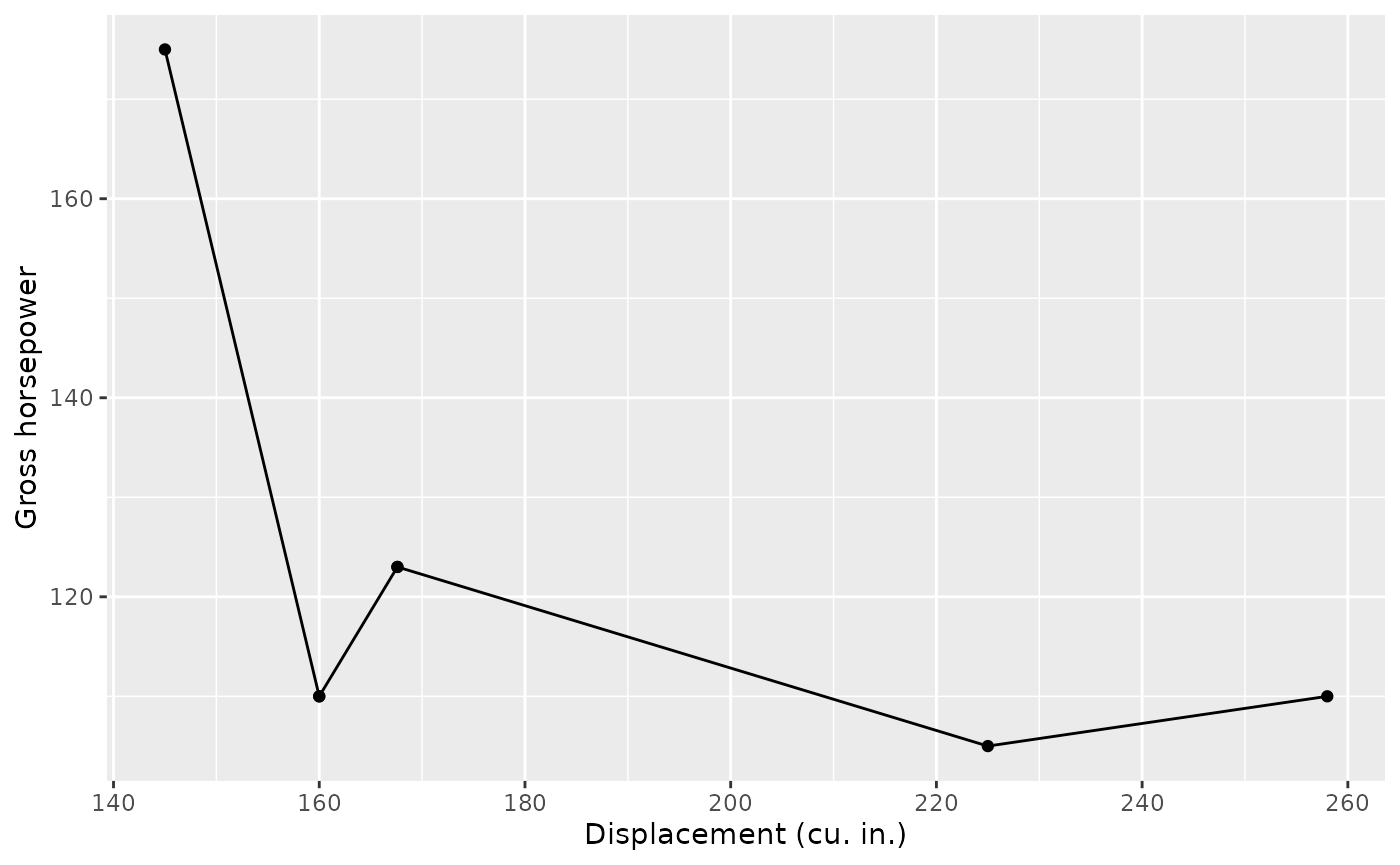
Horsepower by displacement for 6 cars

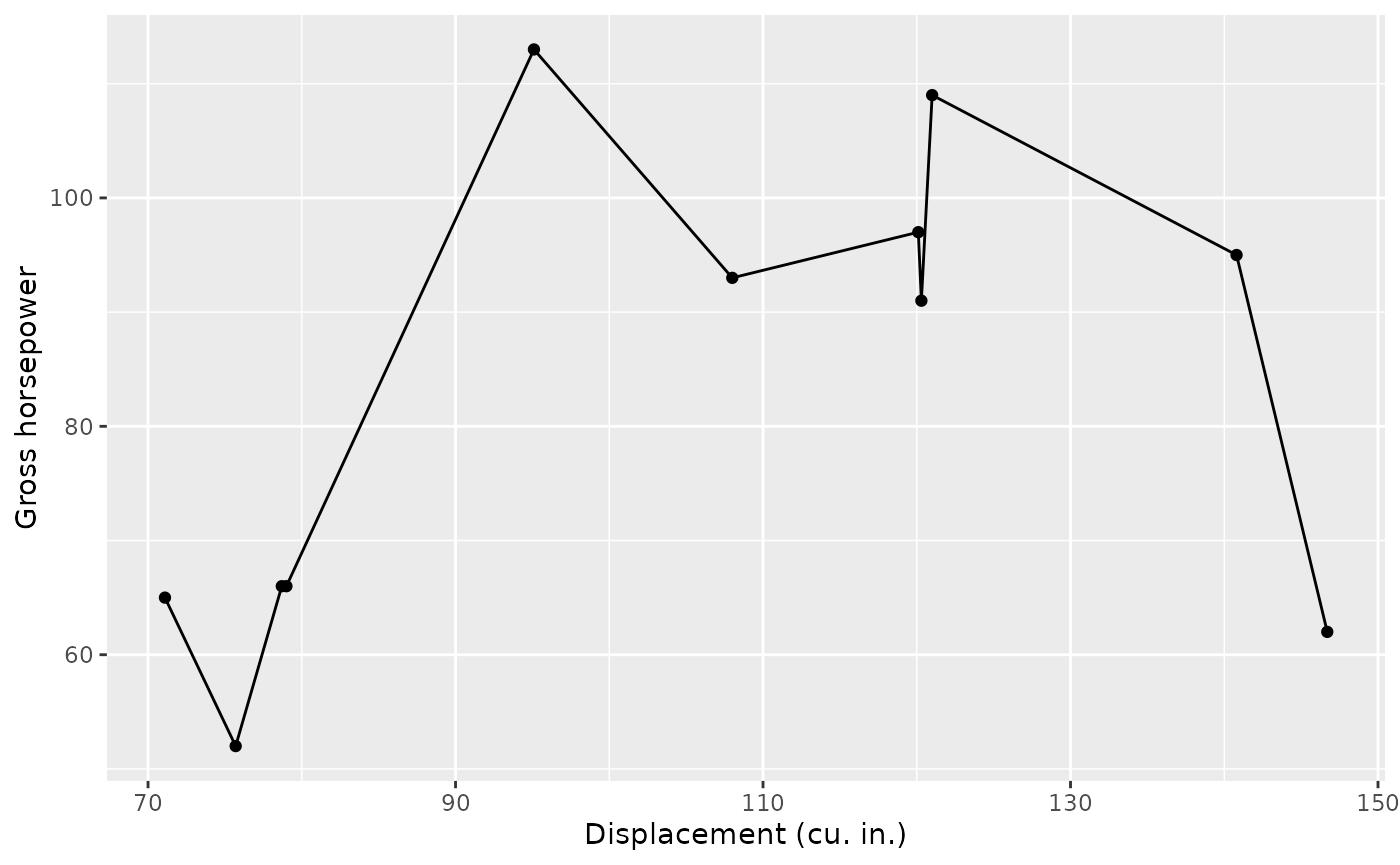
Horsepower by displacement for 4 cars

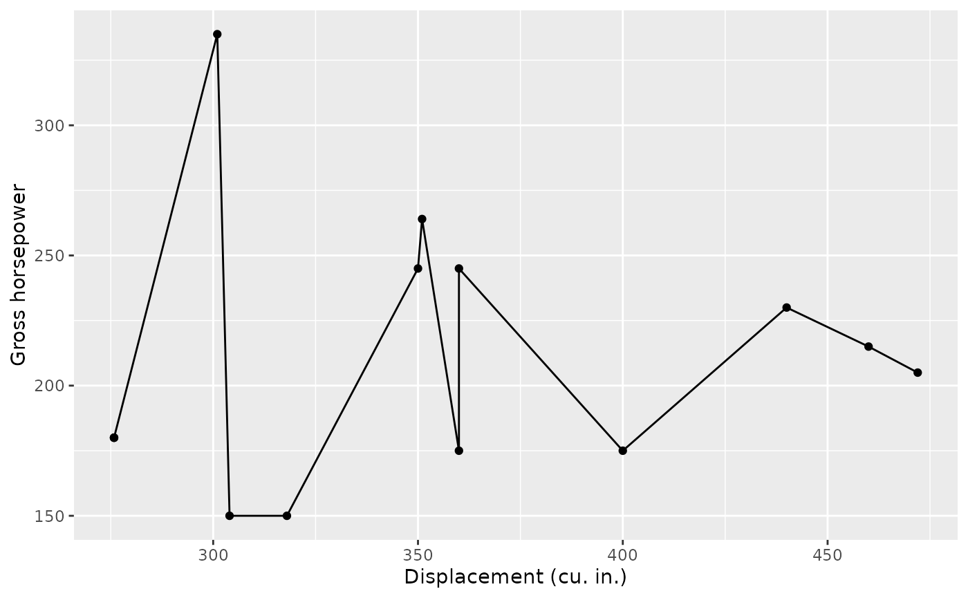
Horsepower by displacement for 8 cars